Published 11/16/2023

NASF/AESF Foundation Research Project #121: Development of a Sustainability Metrics System and a Technical Solution Method for Sustainable Metal Finishing - 14th Quarterly Report

This NASF-AESF Foundation research project report covers the 14th quarter of project work (July-September 2023) at Wayne State University in Detroit.

Edited by: PF Editorial Team

It is widely recognized in many industries that sustainability is a key driver of innovation. Numerous companies, especially large ones who made sustainability as a goal, are achieving clearly more competitive advantages. The metal finishing industry, however, is clearly behind others in response to the challenging needs for sustainable development.

This research project aims to:

Create a metal-finishing-specific sustainability metrics system, which will contain sets of indicators for measuring economic, environmental and social sustainability,
Develop a general and effective method for systematic sustainability assessment of any metal finishing facility that could have multiple production lines, and for estimating the capacities of technologies for sustainability performance improvement,
Develop a sustainability-oriented strategy analysis method that can be used to analyze sustainability assessment results, identify and rank weaknesses in the economic, environmental, and social categories, and then evaluate technical options for performance improvement and profitability assurance in plants, and
Introduce the sustainability metrics system and methods for sustainability assessment and strategic analysis to the industry.

This will help metal finishing facilities to conduct a self-managed sustainability assessment as well as identify technical solutions for sustainability performance improvement.

Progress Report (Quarter 14)

1. Student participation

Mahboubeh Moghadasi, a Ph.D. student in the PI’s group, conducted research in this reporting period. She was financially supported mainly by the PI’s two grants from the National Science Foundation (NSF) and partially by this AESF research project. Her research has been focused on the development of a set of Digital Twins (DTs) using the Physics-Informed Neural Network (PINN) technology. She has made impressive progress in learning PINN fundamentals, writing computer codes using Python - a high-level, general-purpose programming language, and simulating a PINN-based cleaning system model set. The technical component of this report is mainly based on her research, under the PI’s supervision.

Ryan Kitelinger, an undergraduate student of chemical engineering at Florida Institute of Technology, was hired by the PI as an NSF REU fellow to conduct 10-week research in the PI’s lab during the Summer Academy of Sustainable Manufacturing at Wayne State University (June 1 to Aug. 10, 2023). The student learned the fundamentals of electroplating and engineering sustainability through literature survey and conducted computer simulation of a cleaning system model set, assisted by Mahboubeh Moghadasi. The student presented his work during the PI’s lab group’s meetings and the Summer Academy at Wayne State every week. He was recognized as the Best REU Student during the Poster Symposium of the WSU-NSF REU Summer Academy in Sustainable Manufacturing on Aug. 10, 2023.

2. Summary of project activities

Since no publication on the PINN-based DT for electroplating has been identified, we have first provided a general description about the PINN in this report. We then present a set of reduced-order first-principle-based models for parts cleaning, which is a core part of the PINN. It is necessary to state that the PINN-based DT is a very new research area. The purpose of our study in this period is to understand how the PINN works, how to structure it appropriately, and how to train and analyze it effectively in the application to cleaning systems.

2.1 PINN-based digital twinning: basics and architecture

General description. Advanced manufacturing comes into the digital age. Among top strategic digital technologies, Digital Twin (DT) technology has received significant attention. DT is a virtual representation that serves as a digital counterpart of a physical object or system. It is characterized by real-time reflection, interaction and convergence in physical space between historical data and real-time data, and between physical and virtual spaces, and self-evolution. A more recent development in the DT community is the introduction of PINN, which is a type of universal function approximator that can embed the knowledge of any physical laws that govern a given data-set in the learning process. The PINN is an innovative Artificial Intelligence (AI) approach that combines conventional neural network (NN) architectures with the principles of physics (Nascimento, et al., 2020).¹ Unlike regular NNs that rely solely on input data, the PINN ensures that its predictions align with established physical laws, resulting in predictions that are both data-informed and physically consistent. This unique fusion allows for more accurate simulation and the ability to adapt to real-world variations by adjusting physical parameters based on actual system data.

A remarkable advantage of PINN is its ability to handle situations with limited data effectively. Data scarcity is a common challenge in many real-world applications, and PINNs offer an efficient solution to address this issue (Raissi, et al., 2018).² By leveraging its inherent understanding of physical laws, PINNs can make predictions beyond the scope of training data. This capability is particularly valuable in scenarios where data availability is limited or incomplete, which is often the case in electroplating plants. Furthermore, PINNs can provide more transparent and interpretable information, as compared with many other NNs, which are often criticized for their "black box" nature. This transparency allows researchers and practitioners to gain insights when making decisions. PINNs have been successfully applied to solve forward and inverse problems involving nonlinear partial differential equations (PDEs). However, like any technology, the PINN approach has its limitations. The integration of physical laws into the NN architecture increases its computational demands, which may require more robust hardware or extended training periods (Nascimento et al., 2020).¹ Additionally, a solid grasp of relevant physical laws is essential for effective implementation of PINNs. Complex scenarios with unique physical properties may pose integration challenges that need to be carefully addressed. One approach is to use parametric reduced-order models (ROM), instead of PDE, in PINNs (Fu, et al., 2023).³

In pursuit of developing strategies and solutions for electroplating sustainability, we have been studying a PINN-based DT approach. The PINN consists of sets of nonlinear ROMs representing any process, such as alkaline or acid cleaning, single or multiple rinsing, and types of plating.

Architectural aspects. We have explored architectural integration approaches to harness the full potential of PINN when studying electroplating systems. The structure and design of an NN play a pivotal role in determining its efficiency, scalability and overall performance. Given the unique nature of PINN, where physical laws intertwine with data-driven learning, it is imperative to select the appropriate architecture that can seamlessly blend these two realms. The following two primary architectures have been investigated.

PINN as a layer in a Feed-forward Neural Network (FNN). In this setup, a PINN is incorporated as a concluding layer within a standard FNN. Figure 1 shows a schematic diagram of the PINN. While this design ensures a streamlined integration of physical laws into a prediction process, it operates predominantly in a sequential manner. This means that each input passes through the network in a predefined order. While effective in many cases, it might not be able to fully capture the temporal dynamics of certain processes.

Figure 1 - PINN as the last layer of a feedforward neural network (FNN).

PINN as a cell in a Recurrent Neural Network (RNN). This design treats a PINN as an integral cell (Fig. 2a) within an RNN (Fig. 2b). Recurrent networks are known for their ability to remember past information, making them particularly suitable for processes that have temporal sequences or where past events influence future outcomes. By embedding a PINN in this structure, we can ensure that both temporal dynamics and physical laws are considered concurrently during predictions.

2.2 PINN-based DTs for general cleaning systems

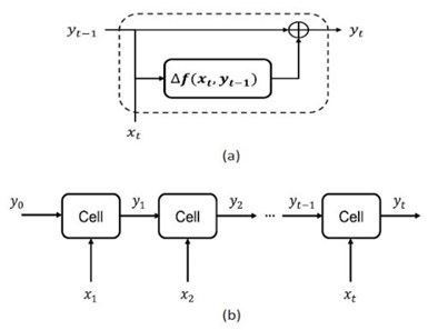
Figure 2 - PINN-embedded RNN: (a) a PINN cell and (b) an RNN configuration.

As the core component of the PINN-based DTs, the integrated, intertwined cleaning system models can provide the following time variant information: (i) the surface cleanness of the parts in cleaning units, and (ii) the chemical concentration dynamics in the units.

Integrated cleaning system DT – Parametric Reduced-Order Models. In a cleaning unit, chemicals are consumed to remove dirt from the surface of parts and then partially lost through drag-out. The amount of dirt on parts is negatively proportional to a dirt removal rate, which is determined by the type of chemicals used, their concentrations, and the type and amount of the dirt on parts. The dirt removal model has the following form.

$A_{p}\frac{dw_{p_{c}}(t)}{dt}=-r_{p_{c}}(t)$ (1)

$r_{p_{c}}(t)=\gamma _{c}(t)C_{a}(t)w_{p_{c}}(t)$ (2)

$\gamma _{c}(t)=\gamma _{0}(1-e^{-\alpha (t-t_{0}^{c})})$ (3)

where 𝐴_𝑝 is the total surface area of the parts in a barrel (cm²); 𝑊𝑝_𝑐 is the amount of dirt on parts (g/cm²); t is time (min); 𝑟𝑝_𝑐 is the dirt removal rate in the cleaning tank (g/min); 𝛾_𝑐 is the looseness of the dirt on parts (cm²·gal-soln/gal-chem·min); 𝐶_a is the chemical concentration in the cleaning tank (gal-chem/gal-soln); 𝛾₀ is the kinetic constant (cm²·gal-soln/gal-chem·min); 𝑡₀^𝑐 is the time when the barrel enters the cleaning tank, and 𝛼 is a constant.

The amount of chemicals in the cleaning unit changes in operation. Its dynamics can be modeled as:

$V_{c}\frac{dC_{a}(t)}{dt}=-\frac{r_{p_{c}}(t)}{\eta }+w_{c}(t)$ (4)

where 𝑉_𝑐 is the capacity of the cleaning tank (gal-soln), and η is the chemical capacity coefficient for dirt removal (g-dirt/gal-chem).

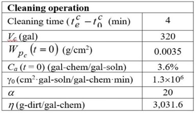
Table 1 - Model parameters in the case study.

Model parameter settings. Model parameters and initial conduction for simulation are listed in Table 1. Note that two parameters (𝛾₀ and η) will vary in operation, which can be adjusted dynamically by the PINN.

2.3 Architecture selection, PINN training and accuracy and runtime study

We have conducted extensive simulation, testing and evaluation using two PINN architectures, the PINN-FNN and the PINN-RNN, for studying alkaline cleaning. Comparing with the results shown in Figs. 3 to 6 (the blue and green curves in each figure), we found that the PINN-RNN was more capable of describing process dynamics, and more importantly of predicting system performance in the future, which was consistent with the governing physical principles.

Figure 4 - Dirt removal dynamics in a cleaning unit (by a PINN-RNN).

Figure 5 - Chemical concentration change in a cleaning unit (by a PINN-FNN).

Figure 6 - Chemical concentration change in a cleaning unit (by a PINN-RNN).

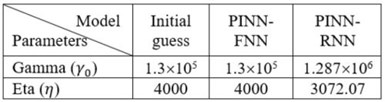
Table 2 – Model parameter adjustment.

Furthermore, when it comes to parameter adjustments for both the DTs, it is evident that the PINN-RNN provides a more accurate estimation of physical parameters (𝛾₀ and η) in Equations (3) and (4) (Table 2). Note that the initial estimate of the parameters used by the PINN-FNN and the PINN-RNN were identical. But the two parameters were automatically adjusted in the PINN-RNN, which made the model estimation and prediction more accurate, while the PINN-FNN had no ability to adjust them, which caused model prediction errors.

PINN-RNN training method. In the realm of employing PINN in our DTs for cleaning, understanding and optimizing model training dynamics is crucial to ensuring the efficacy and accuracy of model-based prediction. The training process adjusts the RNN’s weights and biases to minimize the difference between its predictions and actual observed data. In the PINN simulation, the physical parameters are introduced as weights to the model. In this context, we explored two primary training approaches, namely manual training and automated training utilizing Keras' model.fit() method. Each shows its distinctive advantages and applicability.

Manual training, although computationally intense and often slower, offers nuanced, fine-tuned control over the learning process. This is vital when dealing with models containing multiple parameters to be adjusted. The approach is particularly beneficial for our cleaning system model, which includes two parameters to be adjusted. Manual training allowed us to apply different learning rates for each parameter, which is a strategy that proves to be instrumental in navigating the complex parameter space without violating the physical constraints embedded in the PINN.

On the other hand, if a model has a single parameter to adjust, it is more suitable to use Keras’ model.fit() method. This function performs the training process automatically, adjusting the model's parameters to minimize the loss function efficiently. The singular parameter in a model meant that we could leverage the speed and computational efficiency of model.fit() without sacrificing the model's accuracy or physical consistency.

In essence, the choice of training strategy became inherently tied to the complexity of the model and the number of parameters requiring adjustment. The dual approach, applying manual training for models with multiple parameters and utilizing model.fit() for those with a singular parameter, provided a balanced methodology. This ensures that, across all models, the training process will be both computationally efficient and maintains the vital physical consistency and accuracy that PINN brings to the table.

Solution methods. Two methods were explored for solving the parametric ROMs in Equations 1 to 4. They are the Euler method and the Runge-Kutta method. Our focus was to compare their computational accuracy and computational efficiency.

The Euler method is featured for its simplicity and computational efficiency. If the reduced-order model (ROM) is first-order ODEs (either linear or nonlinear), this method is effective in solution derivation with a relatively low computational cost. The method uses a straightforward iterative process to advance the solution in small increments, making it especially appealing when dealing with real-time simulations or scenarios where computational resources might be limited. However, its solution can sometimes be less accurate than other methods, especially if a system experiences rapid or complex changes.

Conversely, the Runge-Kutta method is often lauded for its accuracy in numerical solutions of ordinary differential equations (ODEs). While typically demanding more computational resources compared to the Euler method, the Runge-Kutta method offers enhanced precision by considering not just the initial point, but also taking midpoints into account in its iterative procedure. This often results in more accurate approximations of solution, especially in scenarios where the system dynamics involve rapid or non-linear changes.

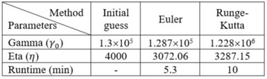
Table 3 – Solution method comparison.

Since the parametric ROM for cleaning are first-order nonlinear models, the Euler method was preferred. This allowed us to achieve a harmonious balance of computational efficiency and solution accuracy. The runtime and accuracy by different methods are summarized in Table 3. Figures 7 to 10 show clearly that the predictions of the dirt removal from parts and the chemical concentration in the cleaning system by the Euler method is better than those by the Runge-Kutta method.

Figure 7 - Dirt removal dynamics using the Runge-Kutta method.

Figure 8 - Dirt removal dynamics using the Euler method.

Figure 9 - Chemical concentration by the Runge-Kutta method.

Figure 10 - Chemical concentration by the Euler method.

Data reliability and data size. Data quality (reliability) and quantity (size) are critical to the successful application of PINN. In an electroplating plant, the collected operational data are often imprecise and may contain various noises. Thus, it is important to assess how well a PINN can navigate through those nuances while still providing dependable and actionable insights.

Outcomes using noisy data set. One of the characteristics of PINN is its deftness in managing data of varied quality. Our study shows that PINN can maintain a notable degree of effectiveness even when the data is not pristine. Whether navigating through clean data, where variables are well-behaved and noise is minimal, or working with noisy data, where variables exhibit random fluctuations, PINN exhibited a robust capacity to make predictions that adhered closely to physical principles. Figure 11 showcases the outcomes using noisy data, vividly illustrating the model’s predictability when facing data with varying degrees of noises.

Figures 11a (above) and 11b (below) - Simulation results obtained using noisy dataset.

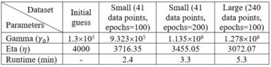
Data size effect. On a parallel front, the effectiveness of PINN was also evaluated with respect to dataset size. In a situation where data was scarce or limited, the intrinsic capability of PINN to leverage physical laws played a significant role. This characteristic ensured that even with a small dataset, PINN could generate predictions that were not just data-driven but also substantiated by established physical principles. It was observed that while the predictive accuracy with a small dataset might not match the precision achieved using larger datasets, the prediction was still quite reliable, maintaining adherence to the underlying physical phenomena. These can be observed through comparing simulation results shown in Figures 12 to 14 and in Table 4.

Figure 12 - Dirt removal dynamics using (a) small and (b) large dataset (epochs=100).

Figure 13 - Chemical concentration dynamics using (a) small and (b) large dataset (epochs=100).

Figure 14 - Dirt removal and chemical concentration dynamics using small dataset (epochs=200).

2.4. Results

Our in-depth study on the PINN with its application using the parametric reduced-order models (ROM) shows that the PINN-RNN, in conjunction with the Euler method for solution derivation is most effective. The extensive simulation shows that the PINN-based digital twinning of the cleaning system can characterize system’s dynamics very precisely, even if there exist data uncertainty and scarcity issues. The key simulation results are listed below.

Single barrel based cleaning. The dirt removal from parts and the chemical concentration changes in a cleaning system are shown in Figs. 12b and 13b, where the actual dynamics (the blue curves) and the predicted curves (the green curves, by the PINN-RNN) are matched very well.

Multiple barrel based cleaning. We used the trained PINN-RNN to simulate the continuous operation of a cleaning system. Assuming that each barrel contains 250 lbs. of parts, and the cleaning time of each barrel is 4 min, we simulated 48 barrels of parts for cleaning in the system. The PINN was tasked with managing a considerably more dynamic and temporally influenced environment. Various initial dirt amounts were considered in the simulation to become closer to a realistic process representation. The simulations result, illustrated in Figs. 15 and 16, underscore a robust and stable prediction curve. This stability was maintained even amidst the intricate and dynamic conditions of managing multiple barrels across varying cleaning stages.

Figure 15 - Dirt removal from the parts surface (Wp_c ) in 48 barrels (250 lbs. of parts per barrel).

Figure 16 - Chemical concentration (C_A) change in the period of cleaning 48 barrels

Automatic adjustment of model parameters. Two model parameters, Gamma and Eta, are key ones to be adjusted, based on the dynamic change of operating conditions.

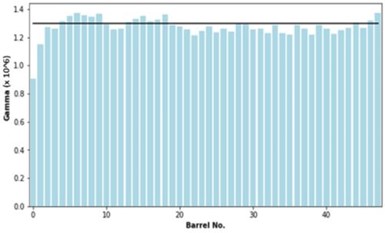
Figure 17 – Adjustment of Gamma parameter values for 48-barrel cleaning.

The PINN-RNN was capable of adjusting them automatically. Figures 17 and 18 show the parameter value adjustment, which contribute to the accurate prediction of parts cleaning quality as well as chemical concentration change in operation.

2.5 Summary

We have significantly gained a much deeper understanding and fundamental knowledge of PINN-based digital twinning for engineering applications. Although the case study on general cleaning is relatively simple, we are now able to construct an effective PINN that contains parametric reduced order models (ROM) and conduct a comprehensive analysis of system performance. The experience gained in the study will be very valuable for our next-step study in the following directions: (1) to develop PINNs for other types of cleaning, rinsing of different configurations and electroplating, and (2) to perform PINN-based dynamic sustainability assessment and decision making for sustainable manufacturing. Hopefully, we will be able to demonstrate that the PINN-based DT technology will eventually be a game-changer for the research and practice for sustainable electroplating.

4. References

1. R.G. Nascimento, K. Fricke and F.A.C. Viana, "A tutorial on solving ordinary differential equations using Python and hybrid physics-informed neural network", Engineering Applications of Artificial Intelligence, 96, 103996 (2020).

2. M. Raissi, P. Perdikaris and G. Karniadakis, "Physics-informed neural networks: a deep learning framework for solving forward and inverse problems involving nonlinear partial differential equations", J. of Computational Physics, 378, 686-707 (2019).

3. J. Fu, D. Xiao, Rui Fu, C. Li, C. Zhu, R. Arcucci and I.M. Navon, “Physics-data combined machine learning for parametric reduced-order modelling of nonlinear dynamical systems in small-data regimes,” Computer Methods in Applied Mechanics and Engineering, 404, 115771 (2023).

6. Past project reports

1. Quarter 1 (April-June 2020): Summary: NASF Report in Products Finishing; NASF Surface Technology White Papers, 84 (12), 14 (September 2020); Full paper: http://short.pfonline.com/NASF20Sep1

2. Quarter 2 (July-September 2020): Summary: NASF Report in Products Finishing; NASF Surface Technology White Papers, 85 (3), 13 (December 2020); Full paper: http://short.pfonline.com/NASF20Dec1

3. Quarter 3 (October-December 2020): Summary: NASF Report in Products Finishing; NASF Surface Technology White Papers, 85 (7), 9 (April 2021); Full paper: http://short.pfonline.com/NASF21Apr1.

4. Quarter 4 (January-March 2021): Summary: NASF Report in Products Finishing; NASF Surface Technology White Papers, 85 (11), 13 (August 2021); Full paper: http://short.pfonline.com/NASF21Aug1

5. Quarter 5 (April-June 2021): Summary: NASF Report in Products Finishing; NASF Surface Technology White Papers, 86 (1), 19 (October 2021); Full paper: http://short.pfonline.com/NASF21Oct2

6. Quarter 6 (July-September 2021): Summary: NASF Report in Products Finishing; NASF Surface Technology White Papers, 86 (4), 19 (January 2022); Full paper: http://short.pfonline.com/NASF22Jan3

7. Quarter 7 (October-December 2021): Summary: NASF Report in Products Finishing; NASF Surface Technology White Papers, 86 (7), 17 (April 2022); Full paper: http://short.pfonline.com/NASF22Apr2

8. Quarter 8 (January-March 2022): Summary: NASF Report in Products Finishing; NASF Surface Technology White Papers, 86 (10), 17 (July 2022); Full paper: http://short.pfonline.com/NASF22Jul2

9. Quarter 9 (April-June 2022): Summary: NASF Report in Products Finishing; NASF Surface Technology White Papers, 87 (1), 17 (October 2022); Full paper: http://short.pfonline.com/NASF22Oct1

10. Quarter 10 (July-September 2022): Summary: NASF Report in Products Finishing; NASF Surface Technology White Papers, 87 (4), 17 (January 2023); Full paper: http://short.pfonline.com/NASF23Jan2

11. Quarter 11 (October-December 2022): Summary: NASF Report in Products Finishing; NASF Surface Technology White Papers, 87 (6), 19 (March 2023); Full paper: http://short.pfonline.com/NASF23Mar1

12. Quarter 12 (January-March 2023): Summary: NASF Report in Products Finishing; NASF Surface Technology White Papers, 87 (10), 20 (July 2023); Full paper: http://short.pfonline.com/NASF23Jul1

13. Quarter 13 (April-June 2023): Summary: NASF Report in Products Finishing; NASF Surface Technology White Papers, 88 (2), TBD (November 2023); Full paper: http://short.pfonline.com/NASF23Nov2

5. About the principal investigator (P.I.)

Dr. Yinlun Huang is a Professor at Wayne State University (Detroit, Michigan) in the Department of Chemical Engineering and Materials Science. He is Director of the Laboratory for Multiscale Complex Systems Science and Engineering, the Chemical Engineering and Materials Science Graduate Programs and the Sustainable Engineering Graduate Certificate Program, in the College of Engineering. He has ably mentored many students, both Graduate and Undergraduate, during his work at Wayne State.

He holds a Bachelor of Science degree (1982) from Zhejiang University (Hangzhou, Zhejiang Province, China), and M.S. (1988) and Ph.D. (1992) degrees from Kansas State University (Manhattan, Kansas). He then joined the University of Texas at Austin as a postdoctoral research fellow (1992). In 1993, he joined Wayne State University as Assistant Professor, eventually becoming Full Professor from 2002 to the present. He has authored or co-authored over 220 publications since 1988, a number of which have been the recipient of awards over the years.

His research interests include multiscale complex systems; sustainability science; integrated material, product and process design and manufacturing; computational multifunctional nano-material development and manufacturing; and multiscale information processing and computational methods.

He has served in many editorial capacities on various journals, as Co-Editor of the ASTM Journal of Smart and Sustainable Manufacturing Systems, Associate Editor of Frontiers in Chemical Engineering, Guest Editor or member of the Editorial Board, including the ACS Sustainable Chemistry and Engineering, Chinese Journal of Chemical Engineering, the Journal of Clean Technologies and Environmental Policy, the Journal of Nano Energy and Power Research. In particular, he was a member of the Editorial Board of the AESF-published Journal of Applied Surface Finishing during the years of its publication (2006-2008).

He has served the AESF and NASF in many capacities, including the AESF Board of Directors during the transition period from the AESF to the NASF. He served as Board of Directors liaison to the AESF Research Board and was a member of the AESF Research and Publications Boards, as well as the Pollution Prevention Committee. With the NASF, he served as a member of the Board of Trustees of the AESF Foundation. He has also been active in the American Chemical Society (ACS) and the American Institute of Chemical Engineers (AIChE).

He was the 2013 Recipient of the NASF William Blum Scientific Achievement Award and delivered the William Blum Memorial Lecture at SUR/FIN 2014 in Cleveland, Ohio. He was elected AIChE Fellow in 2014 and NASF Fellow in 2017. He was a Fulbright Scholar in 2008 and has been a Visiting Professor at many institutions, including the Technical University of Berlin and Tsinghua University in China. His many other awards include the AIChE Research Excellence in Sustainable Engineering Award (2010), AIChE Sustainable Engineering Education Award (2016), the Michigan Green Chemistry Governor’s Award (2009) and several awards for teaching and graduate mentoring from Wayne State University, and Wayne State University’s Charles H. Gershenson Distinguished Faculty Fellow Award.

* Dr. Yinlun Huang, Professor

Dept. of Chemical Engineering and Materials Science

Wayne State University

Detroit, MI 48202

Office: (313) 577-3771

E-mail: yhuang@wayne.edu